
FINANCIAL MANAGEMENT
Capital Structure Theories
Capital structure may be defined as a combination of debt capital and equity capital of a corporate entity (business firm). Optimum capital structure may be defined as that capital structure or combination of debt capital and equity capital which leads to the minimum overall cost of capital (k o) and maximum value of the business firm (corporate entity).
The four major capital
structure theories are:
1. Net income approach,
2. Net operating income approach,
3. Modigliani – Miller (MM) approach,
4. Traditional approach.
General
assumptions for capital structure theories:
1.
There are only
two sources of funds used by a business firm: perpetual risk free debt and
ordinary (equity) shares.
2.
The Dividend Payout Ratio is 100%.
3.
The firm’s total assets are
given and do not change (i.e. Total Assets are constant).
4.
The firm’s total
capital (i.e. equity + debt) remains constant. It can change its degree
of financial leverage (i.e. capital structure) either by selling shares and
using the proceeds to retire debentures or by raising more debt capital to
reduce the equity capital.
5.
The operating profits
(EBIT) are not expected to grow (i.e. EBIT is constant).
6.
All investors have the same
expectation of the firm’s future EBIT.
7.
The firm’s business risk is
constant over a period of time and is assumed to be independent of its capital
structure and financial risk.
8.
The firm’s life is perpetual.
Net income approach
According to the net income (NI) approach the capital
structure decision is relevant to the valuation of the firm. A change
in the capital structure will lead to a corresponding change in the overall
cost of capital as well as the total value of the firm. If the degree of
financial leverage as measured by the ratio of debt to equity is increased the
weighted average cost of capital will decline, while the total value of the
firm as well as the market price of equity shares will increase. Conversely, a
decrease in the degree of financial leverage will cause an increase in the
overall cost of capital and a decline both in the total value of the firm as
well as the market price of equity shares.
Specific
assumptions:
1.
Cost of debt is less than
cost of equity (i.e. k d < ke).
2.
Due to change in the degree
of financial leverage, there will be no change in either the cost of debt or
the cost of equity (i.e. k d and ke are
constant).
3.
There are no
corporate taxes.
4.
Any change in the degree of
financial leverage of the firm does not change the risk perception of the
investors about the firm.
Net operating income approach
According to the net operating income (NOI) approach
the capital
structure decision is irrelevant to the valuation of the firm. A change
in the capital structure will not lead to any change in the total value of the
firm and the market price of equity shares, as the overall cost of capital is
independent of the degree of financial leverage (i.e. capital structure).
Specific
assumptions:
1.
The overall cost of capital
(k o) and cost of debt (k d) of the firm remain constant
for all the degrees of financial leverage i.e. for all the capital structures (k o
and k d are constant).
2.
Cost of debt is less than
cost of equity (i.e. k d < ke).
3.
The market
value of equity (S) is a residual value which is determined by
deducting the total market value of debt (B) from
the total market value of the firm (V). Symbolically, S = V – B.
4.
The cost of equity capital
(ke) increases with the increase in the degree of financial leverage
(ratio of debt to equity).
5.
There are no
corporate taxes.
Modigliani – Miller approach
The Modigliani – Miller (MM) approach in respect of
the relationship between the capital structure, cost of capital and value of
the firm is akin to the NOI approach. The propositions of the MM approach may
be stated as follows:
Initial proposition (if
there are no corporate taxes):
The overall cost of capital (k o) and the
value of the firm (V) are independent of its capital structure. K o
and V are constant for all degrees of financial leverage (i.e. capital
structures).
Modified proposition (if
there is corporate taxes):
(i) Overall cost of capital (k o) can be
lowered by increasing the degree of financial leverage of the firm;
(ii) Value of the firm (V) can be increased by
increasing its degree of financial leverage.
Specific
assumptions (for initial proposition):
MM proposition that weighted average cost of capital
(k o) and the value of the firm (V) are constant irrespective of the
type of capital structure is based on the following assumptions:
1.
There is no
corporate tax in the system.
2.
Capital markets are perfect implying that –
(a) Securities are infinitely divisible,
(b) Investors are free to buy or sell securities,
(c) Investors can borrow without restrictions on the same
terms and conditions as firms can,
(d) There are no transaction costs,
(e) Each investor has the same information which is
readily available to him without cost,
(f) Investors are rational and behave accordingly.
3.
All investors have the same
expectation of the firm’s net operating income (EBIT) on the basis of which the
value of the firm is to be determined.
4.
Business risk is equal
among all the firms with similar operating environment.
5.
The dividend payment ratio is 100%.
Traditional approach
The traditional approach is midway between the NI and
NOI approaches. It partakes of some features of both these approaches. While
the traditional approach supports the proposition that the capital structure
decision is relevant to the overall cost of capital and total value of the
firm, it does not subscribe to the view that the value of the firm will
necessarily increase for all increases in the degree of financial leverage at
all levels of activity. The traditional approach, on the contrary, has divided
the impact of the degree of financial leverage on the overall cost of capital
in three stages as follows:
First Stage:
At the initial stage, the cost of equity capital
remains constant or rises slightly with an increase in debt capital. Again, at
this stage, the cost of debt capital also remains constant or rises negligibly
since the market views the use of debt as a reasonable policy. As a result, the
weighted average cost of capital will fall and the value of the firm will
increase with an increase in debt-equity ratio.
Second Stage:
After a certain degree of financial leverage, the cost
of equity capital will tend to rise because of the increased risk perception of
the equity shareholders. At this stage, the increase in the cost of equity (due
to added financial risk arising out of higher degree of financial leverage)
will just offset the benefit of using cheaper debt capital. It will continue up
to a certain range of the degree of financial leverage. Hence, within
this range of the degree of financial leverage, the weighted average cost of
capital will remain unchanged. The weighted average cost of capital will be the
minimum at this stage and hence, the value of the firm will be the maximum.
So, this range of the degree of financial leverage would be regarded as the
optimum degree of financial leverage.
Third Stage:
At this stage, if the degree of financial leverage of the firm is increased beyond the range as shown in the second stage, the risk perception of the debt holders will also rise. At the same time, the cost of equity capital will rise at higher pace because the equity shareholders will perceive a high degree of financial risk and hence, demand a higher equity capitalisation rate. Thus, the rise in the cost of equity capital will offset the advantage of low-cost debt capital. As a result, the weighted average cost of capital will rise and the value of the firm will decrease with an increase in debt-equity ratio.
Important Formulas
|
|
Net Income
(NI) Approach |
|
|
1 |
Market value of the firm, V |
= S + B |
|
2 |
Market value of each Eq. share, Po |
= EPS1 ÷ ke [EPS1 = Expected earnings per
share] |
|
3 |
Market value of the Eq. capital, S |
[(EBIT – I) × (1 – t)] ÷ ke |
|
4 |
Market value of the debt capital, B |
= I ÷ k d [Here, k d = Before-tax cost of
debt] |
|
5 |
Overall cost of capital, k o |
= k d x (B ÷ V) + ke x
(S ÷ V) [Here, k d = After-tax cost of
debt] |
|
|
|
|
|
|
Net Operating
Income (NOI) Approach |
|
|
6 |
Market value of the firm, V |
= EBIT ÷ ko |
|
7 |
k o |
= EBIT ÷ V |
|
8 |
Market value of the debt capital, B |
= I ÷ k d [Here, k d = Before-tax cost of
debt] |
|
9 |
Market value of total Eq. capital, S |
= V – B |
|
10 |
Cost of equity capital, k e |
= [(EBIT – I) ÷ S |
|
11 |
Cost of equity capital, k e |
= k o + (k o – k d)
(B ÷ S) [Here, k o and k d are
constant] |
|
|
|
|
|
|
Modigliani –
Miller (MM) Approach (Assuming
existence of corporate tax) |
|
|
12 |
Value of unlevered firm, VU |
= [EBIT x (1 – t)] ÷ k o |
|
13 |
Value of levered firm, VL |
= VU + B x t |
|
14 |
Value of levered firm, VL |
= [{EBIT x (1 – t)} ÷ k o] + B x t [Here, Ko = ke] |
|
15 |
k o (unlevered firm) |
= ke |
|
16 |
k o (levered firm) |
= k d x (B ÷ V) + ke x
(S ÷ V) |
|
17 |
ke (levered firm) |
= [(EBIT – I) (1 – t)] ÷ S = EAT ÷ S [Here, S = VL – B] |
|
18 |
K d |
= After-tax cost of debt |
Arbitrage Process
The term arbitrage refers to an act of selling an
asset/security in one market (at higher price) and buying it in another (at
lower price), while absolute amount of return to the investor remains the same. As a result, equilibrium is restored in the market
price of the security in different markets. In relation to the Modigliani -
Miller (MM) approach, the essence of the arbitrage process is “selling
of securities of one firm at higher prices and purchasing of securities of
another firm at lower prices maintaining the same absolute amount of return
even after switching of the investment from one firm to another”, where
the firms, belonging to the same risk class, are identical in all respects
except for the difference in their respective capital structures.
According to Modigliani − Miller (MM) approach the
market value of a firm (V) is independent of its capital structure. In other
words, as an extension of the MM approach, it can be said that two firms
belonging to the same risk class and identical in all respects except for the
difference in their respective capital structures cannot have different market
values. Modigliani and Miller also said that the values of the homogeneous
firms, which differ only in respect of leverage, cannot be different, because
of the operation of arbitrage. The investors of the firm whose value is higher
(levered firm) will sell their shares and instead buy the shares of the firm
whose value is lower (unlevered firm). In this arbitrage process the investors
will be able to earn the same return at lower outlay with the same perceived
risk i.e. they would be better off because an investor would borrow at the same cost and in the same proportion of the degree of
leverage present in the high value (levered) firm, shares of which he would
be selling. The behaviour of the investors will have the effect of - (i) increasing
the share prices (value) of the firm whose shares are being purchased; and (ii)
lowering the share prices (value) of the firm whose shares are being sold. This
will continue till the market values (V) of the two firms become identical and
the overall costs of capital (k o) are the same. The use of debt by
the investor for the arbitrage process is called home-made leverage or personal
leverage.
Part B
Illustration: 1
A company’s expected annual net
operating income (EBIT) is Rs 50,000. The company has Rs 2, 00,000 10%
debentures. The equity capitalisation rate (Ke) of the company is 12.5%. Find
the value of the firm and overall cost of capital under Net Income approach.
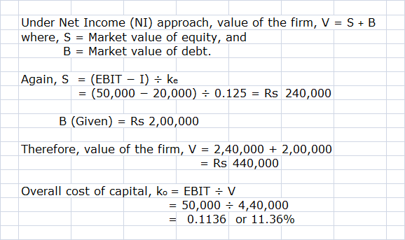
Illustration: 2
Assuming no taxes and given the earnings before
interest and taxes (EBIT), interest (I) at 10% and equity capitalisation rate (Ke) below, calculate the total market value of each firm
under Net Income Approach:
|
Firms |
EBIT
(Rs) |
Interest
(Rs) |
ke |
|
X |
2,00,000 |
20,000 |
12% |
|
Y |
3,00,000 |
60,000 |
16% |
|
Z |
5,00,000 |
2,00,000 |
15% |
|
W |
6,00,000 |
2,40,000 |
18% |
Also determine the weighted average
cost of capital (k o) for each firm.

Illustration: 3
The existing capital structure of XYZ Ltd. is as under:
|
|
Rs |
|
Equity Shares of Rs 100 each |
40,00,000 |
|
Retained Earnings |
10,00,000 |
|
9% Preference Shares |
25,00,000 |
|
7% Debentures |
25,00,000 |
The existing rate of return on the
company’s capital is 12% and the income-tax rate is 50%.
The company requires a sum of Rs 25, 00,000 to finance
an expansion programme for which it is considering the following alternatives:
i.
Issue of 20,000 equity shares at a premium of Rs 25
per share.
ii.
Issue of 10% preference shares.
iii.
Issue of 8% debentures.
It is estimated that the PE ratios in the cases of
equity, preference and debenture financing would be 20, 17 and 16 respectively.
Which of the above alternatives would
you consider to be the best?

Illustration: 4
XL Limited provides you with following figures:
|
|
Rs |
|
Profit (EBIT) |
2,60,000 |
|
Less: Interest on Debentures @ 12% |
60,000 |
|
EBT |
2,00,000 |
|
Less: Income tax @ 50% |
1,00,000 |
|
EAT / PAT |
1,00,000 |
|
Number of Equity shares (of Rs 10 each) |
40,000 |
|
Earnings per share (EPS) |
2.50 |
|
Ruling market price of each equity
share |
25 |
|
P/E Ratio (i.e. Market Price
/ EPS) |
10 |
The Company has undistributed reserves of Rs 6,
00,000. The company now needs Rs 2, 00,000 for expansion. This amount will earn
at the same rate as funds already employed. You are informed that a debt equity
ratio Debt / (Debt+ Equity) more than 35% will push the P/E Ratio down to 8 and
raise the interest rate on additional amount borrowed to 14%.
You are required to ascertain the probable price of
the share –
i. If the
additional funds are raised as debt; and
ii. If the amount
is raised by issuing equity shares.

Illustration:
5
From the following data find out the value of each
firm and value of each equity share as per the Modigliani-Miller approach:
|
|
P |
Q |
R |
|
EBIT |
13,00,000 |
13,00,000 |
13,00,000 |
|
No. of shares |
3,00,000 |
2,50,000 |
2,00,000 |
|
12% debentures |
|
9,00,000 |
10,00,000 |
Every firm expects a 12%
return on investment.

Illustration:
6
Companies X and Y are in the same risk class, and are
identical in every fashion except that Company X uses debt while Company Y does
not. The levered firm has Rs 9, 00,000 debentures, carrying 10% rate of
interest. Both the firms earn 20% before interest and taxes on their total
assets of Rs 15 lakhs. Assume perfect capital markets, rational investors and
so on; a tax rate of 50% and capitalisation rate of 15% for an all equity
company.
a) Compute the value of firms X
and Y using the net income (NI) approach.
b) Compute the value of each firm
using the Modigliani – Miller (MM) approach.
c) Using the MM approach,
calculate the overall cost of capital (k o) for firms X and Y.
d) Which of these two firms has an
optimal capital structure according to the MM approach? Why?

Illustration: 7
Merry
Ltd. has earnings before interest and taxes (EBIT) of Rs 30, 00,000 and a 40% tax rate. Its required rate of
return on equity in the absence of borrowing is 18%. What is the value of the
company under Modigliani – Miller approach (i) with no leverage; ii) with Rs 40,00,000
in debt, and iii) with Rs 70,00,000 in debt?
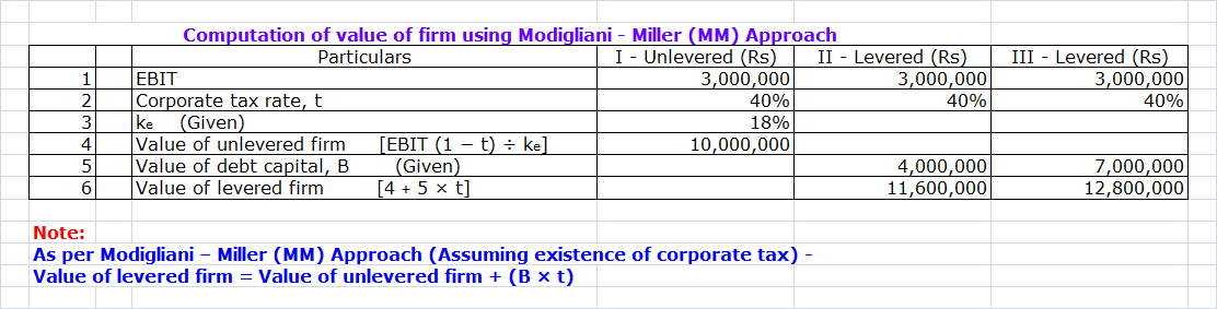
Illustration: 8
Companies X and Y are identical in all respects including
risk factors except for debt/equity ratio. Company X is having issued 10%
debentures of Rs 18 lakhs while Company Y has issued only equity. Both
the companies earn 20% before interest and taxes on their total assets of Rs 30
lakhs.
Assuming a tax rate of 50% and capitalisation rate of
15% for an all-equity company, compute the value of companies X and Y using i)
Net Income Approach and ii) Net Operating Income Approach.
Solution: 8

No comments:
Post a Comment