Business Statistics - Measures of Dispersion (Formulas and Selected Problems and Solutions)

 

Business Statistics

Measures of Dispersion

(Formulas and Selected Problems and Solutions)

 

Part A:

In Part A you will find Formulas of different measures of Dispersion including the important properties of standard deviation.

Part B:

In Part B you will find seventeen selected problems with solutions.

Part A

A measure of dispersion is designed to state numerically the extent to which individual observations vary around the average. There are several measures of dispersion under the two broad categories as follows:

A.       Absolute Measures:

1.       Range,

2.       Quartile Deviation

        (Also known as 'Semi-Interquartile Range')

3.       Mean Deviation About Mean,

4.       Mean Deviation About Median, and

5.       Standard Deviation.

 

B.       Relative Measures:

1.       Coefficient of Range

2.       Coefficient of Quartile Deviation,

3.       Coefficient of M.D. About Mean,

4.       Coefficient of M.D. About Median, and

5.       Coefficient of Variation.

 

Note: Mean Deviation (M.D.) is usually calculated about arithmetic mean, and hence if it’s only ‘Mean Deviation’, it refers to M.D. About Mean only.

 

 

Formulas

 

1.           Range

= Largest Value (L) – Smallest Value (S)

2.           Coefficient of Range

= [(L – S) ÷ (L + S)] × 100

3.           Quartile Deviation = ½ (Q3 – Q1)

4.          Coefficient of Quartile Deviation (1^st Formula)

= [(Q3 – Q1) ÷ (Q3 + Q1)] × 100

5.          Coefficient of Quartile Deviation (2^nd Formula)

= [Quartile Deviation ÷ Median) × 100

6.          Mean Deviation About Mean (For Simple Distribution)

= [∑Mod (x_i – Mean)] ÷ n

7.           Mean Deviation About Mean (For Frequency Distribution)

= [∑f_i {Mod (x_i – Mean)}] ÷ ∑f_i

8.     Mean Deviation About Median (For Simple Distribution)

= [∑Mod (x_i – Median)] ÷ n

9.   Mean Deviation About Median (For Frequency Distribution)

= [∑f_i {Mod (x_i – Median)}] ÷ ∑f_i

10.      Coefficient of M.D. About Mean

= [M.D. About Mean ÷ Mean] × 100

11.      Coefficient of M.D. About Median

= [M.D. About Median ÷ Median] × 100

 

Standard Deviation

 

12.      For Simple Distribution (1^st Formula)

= √ [∑ {(x_i – Mean) ^2} ÷ n]

13.      For Simple Distribution (2^nd Formula - Direct Method)

= √ [{∑ (x_i^2) ÷ n} – {(∑x_i ÷ n) ^2}]

14. For Simple Distribution (3^rd Formula – Short-Cut Method)

= √ [{∑ (d_i^2) ÷ n} – {(∑d_i ÷ n) ^2}]

[Here, d_i = x_i – A; A = Assumed Mean (as near as possible to the true mean)]

15.     For Simple Distribution (4^th Formula – Step-Deviation Method)

= √ [{∑ (D_i^2) ÷ n} – {(∑D_i ÷ n) ^2}] × c

[Here, D_i = (x_i – A)/c; A = Assumed Mean (as near as possible to the true mean); c = Common factor]

16.         For Frequency Distribution (1^st Formula)

= √ [∑ {f_i (x_i – Mean) ^2} ÷ ∑f_i]

17.  For Frequency Distribution (2^nd Formula - Direct Method)

= √ [{∑f_i (x_i^2) ÷ ∑f_i} – {(∑f_ix_i ÷ ∑f_i) ^2}]

18.      For Frequency Distribution (3^rd Formula – Short-Cut Method)

= √ [{∑f_i (d_i^2) ÷ ∑f_i} – {(∑f_id_i ÷ ∑f_i) ^2}]

[Here, d_i = x_i – A; A = Assumed Mean (value of that observation or that mid-value which has the highest frequency)]

19.  For Frequency Distribution (4^th Formula – Step-Deviation Method)

= √ [{∑f_i (D_i^2) ÷ ∑f_i} – {(∑f_iD_i ÷ ∑f_i) ^2}] × c

[Here, D_i = (x_i – A)/c; A = Assumed Mean (value of that observation or that mid-value which has the highest frequency); c = Common factor or common width]

20.       Coefficient of Variation (i.e. Coefficient of SD)

        = (SD ÷ AM) × 100

21.       Variance = SD^2

 

Important note:

Formula of SD for simple frequency distribution and grouped frequency distribution under all the above four methods are same. Only thing to be remembered is that in case of grouped frequency distribution x_i will be the mid-values of the class intervals.

Important Properties of Standard Deviation

 

1.       If y = x ± c where 'c' is a constant,

SD of y = SD of x

i.e. σ_y = σ_x

2.       If x = c + dy where 'c' and 'd' are constants,

σ_x = (Mod 'd') × σ_y

3.       √ [1/n∑ (x_i – Mean of x) ^2] ≤ √ [1/n∑ (x_i – A) ^2] whatever be the value of A.

 

SD of Composite Group

Composite SD

= √ [(N₁σ₁^2 + N₂σ₂^2 + N₁d₁^2 + N₂d₂^2) ÷ (N₁ + N₂)]

 

[Here,

x_i = Observations of Group 1

y_i = Observations of Group 2

d₁ = Mean of Group 1 – Composite Mean

d₂ = Mean of Group 2 – Composite Mean

σ₁ = SD of Group 1

σ₂ = SD of Group 2

Composite mean = [(∑fx) + (∑fy)]/ (N1 + N2)

= [(N1*Mean of x) + (N2*Mean of y)]/ (N1 + N2)

n1 = Total number of observations of Group- 1

n2 = Total number of observations of Group- 2

N1 = Total frequency of Group- 1

N2 = Total frequency of Group- 2]

Part B

Statistics

Measures of Dispersion

Selected Problems and Solutions

 

Problem: 1

Calculate Standard Deviation and Coefficient of S.D. for the following data:

x	f
2	5
4	15
6	20
8	25
10	25
12	20
15	8

 

Solution: 1

Problem: 2

From the following frequency distribution calculate S.D. and Variance:

Annual Salary (Rs ’000)	No. of people
700 – 799	4
800 – 899	7
900 – 999	8
1000 – 1099	10
1100 – 1199	12
1200 – 1299	17
1300 – 1399	13
1400 – 1499	10
1500 – 1599	9
1600 – 1699	7
1700 – 1799	2
1800 – 1899	1

 

Solution: 2

Problem: 3

Calculate the population variance for the following set of grouped data:

Class	Frequency
0 – 199	8
200 – 399	13
400 – 599	20
600 – 799	12
800 – 999	7

 

Solution: 3

Problem: 4

Calculate the mean deviation from the following data, relating to heights (to the nearest inch) of 100 children:

 

Height (inches)	No. of Children
60	2
61	0
62	15
63	29
64	25
65	12
66	10
67	4
68	3

 

Solution: 4

Problem: 5

Find the standard deviation for the distribution given below:

x	Frequency
1	10
2	20
3	30
4	35
5	14
6	10
7	2

 

Solution: 5 

Problem: 6

Find the mean and the S.D. from the following frequency distribution:

Weight (lbs.)	Number of Persons
131 – 140	2
141 – 150	5
151 – 160	4
161 – 170	9
171 – 180	7
181 – 190	5
191 – 210	3
211 – 240	1

 

Solution: 6

Problem: 7

Find mean deviation for the following frequency distribution:

Variable	Frequency
3	2
5	7
7	10
9	9
11	5
13	1

 

Solution: 7 

Problem: 8

Find the S.D. from the following table giving the age distribution of 540 members of a Parliament:

Age in Years	No. of Members
30	64
40	132
50	153
60	140
70	51

 

Solution: 8

Problem: 9

Find the S.D. from the following frequency distribution:

Weight (lbs.)	No. of Boys
120 – 124	12
125 – 129	25
130 – 134	28
135 – 139	15
140 – 144	12
145 – 149	8

 

Solution: 9

Problem: 10

Find the standard deviation of the following distribution:

Turnover (Rs ’000 p.a.)	No. of Firms
50 – 100	5
100 – 150	8
150 – 200	9
200 – 250	12
250 – 300	18
300 – 350	23
350 – 400	17

 

Solution: 10

Problem: 11

Compute the S.D. of income from the following distribution:

Income (Rs)	No. of Earners
Below 200	25
200 – 399	72
400 – 599	47
600 – 799	22
800 – 999	13
1000 – 1199	7

 

Solution: 11

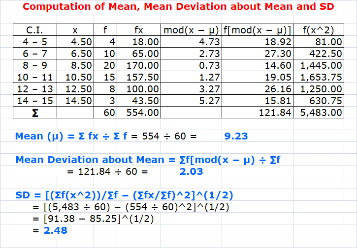
Problem: 12

Compute the arithmetic mean, mean deviation about the mean and standard deviation for the following data:

Scores	Frequency (f)
4 – 5	4
6 – 7	10
8 – 9	20
10 – 11	15
12 – 13	8
14 – 15	3

 

Solution: 12

Problem: 13

From the market prices of shares x and y below find out which is more stable in value:

x	y
35	108
54	107
52	105
53	105
56	106
58	107
52	104
50	103
51	104
49	101

 

Solution: 13

Problem: 14

You are given the distribution of wages in two factories X and Y as follows:

Wages (Rs)	No. of Workers (X)	No. of Workers (Y)
50 – 100	2	6
100 – 150	9	11
150 – 200	29	18
200 – 250	54	32
250 – 300	11	27
300 – 350	5	11

 

State in which factory the wages are more variable.

 

Solution: 14

Problem: 15

Calculate the Coefficient of Variation from the following data, showing Grades of 100 students in M.A. Mathematics.

Grades	No. of Students
30 – 39	2
40 – 49	3
50 – 59	11
60 – 69	20
70 – 79	32
80 – 89	25
90 – 99	7

 

Solution: 15

Problem: 16

The Mean and the S.D. of a sample of 100 observations were calculated as 40 and 5.1 respectively, by a student who by mistake took one observation as 50 instead of 40. Calculate the correct Mean and S.D.

 

Solution: 16

 

Problem: 17

For a distribution of 280 observations mean and standard deviation were found to be 54 and 3 respectively. On checking it was discovered that two observations, which should correctly read as 62 and 82, had been wrongly recorded as 64 and 80 respectively. Calculate the correct values of mean and standard deviation.

 

Solution: 17