Strategic Financial Management - Risk Analysis in Capital Budgeting

Strategic Financial Management

Risk Analysis in Capital Budgeting

 

Part A:

In this part various alternative techniques /approaches for dealing with risks and uncertainties in capital investment decisions along with different important relevant formulas have been explained and discussed in details.

 

Part B:

In this part you will find 11 Illustrations with Solutions.

Part A

Introduction

A financial manager while making an investment decision may confront three alternative situations relating to the possible risk or uncertainty level of the decisions. The three situations are:

 

1	Making decisions under complete certainty,
2	Making decisions under complete uncertainty, and
3	Making decisions under risk.

 

Decision making under complete certainty implies that the manager is fully aware of all the states of nature (i.e., possible events not under the control of the firm) available and expected payoffs from the strategies under consideration for each of the states of nature. Since all the outcomes are fully known to the manager, he can construct a pay-off matrix for all the states of nature and can select the best possible strategy with the maximum pay-off.

 

Unfortunately, in a real dynamic business world, such a situation hardly prevails and what a financial manager can actually confront is either a situation of complete uncertainty or a situation of risk.

 

While dealing with risk and uncertainties in capital investment decisions, financial managers resort to various alternative techniques. Some of the important techniques are:

1	Certainty Equivalent (CE) Approach
2	Risk Adjusted Discount Rate (RADR) Approach
3	Expected NPV and Standard Deviation of NPV Approach (also known as Hillier Model)
4	Normal Probability Distribution (NPD) Approach
5	Simulation Approach

 

Certainty Equivalent Approach

Under this approach cash inflows after tax (CIATs), i.e. risky cash flows over the life of a project, are converted into certainty equivalent cash flows. Certainty equivalent cash flows are derived through multiplying the estimated risky cash flows (CIATs) of the future periods by Certainty Equivalent Co-efficient (CEC) of the respective periods. Certainty Equivalent Co-efficient is calculated based on the risk perceived by the decision maker.

 

The certainty equivalent cash flows are then discounted with the risk-free discount rate to arrive at their present values and make a decision on the acceptance of the project under consideration.

 

The Certainty Equivalent Co-efficient (CEC) ranges between 0 and 1. The higher the co-efficient, the higher is the confidence of the management on the forecasted cash flows. A CEC of unity indicates that the management is completely certain about the cash flows to be realised. On the other hand, a CEC of zero will indicate that the management is highly doubtful about the realisation of the estimated cash flows. Generally, the CECs are high for the initial years and decreases in the later years of the project as the risk will be higher in the later years.

 

Steps to calculate NPV under the Certainty Equivalent Approach:

1	Estimate the cash inflows, i.e. risky cash inflows of the project (CIATt)
2	Multiply CIATt by Certainty Equivalent Coefficient (αt) to determine the certainty equivalent cash inflows (αt × CIATt)
3	Calculate total present value of the certainty equivalent cash inflows by applying the risk-free discount rate (r)
4	Total PV of Certainty Equivalent Cash Inflows = ∑(t = 1 to n) [(αt × CIATt) ÷ (1 + i)t]
5	i = r ÷ 100
6	NPV = Total PV of Certainty Equivalent Cash Inflows – Initial Investment

 

If NPV is positive, the project is acceptable.

Risk Adjusted Discount Rate Approach

An investor usually expects higher return for taking higher risks. The same concept is used in the Risk Adjusted Discount Rate approach of dealing with risk in the context of capital investment decisions. If the risk of a new project is similar to the existing projects, the weighted average cost of capital (WACC) is used as the discounting rate. But, if the project involves higher risk, a higher discounting rate is used for adjusting the risk involved. The additional discounting rate over and above the weighted average cost of capital is known as risk premium. The risk premium takes care of the project risk and may vary from project to project depending on the risk involved in it. So, the risk adjusted discount rate is the aggregate of weighted average cost of capital and risk premium. Due to increase in the discount rate, present value of the cash flows from the project will be less and the value of NPV and PI of the project will also be reduced. This conservative estimate of benefits will take care of risk and uncertainties. The formula for risk adjusted discount rate (RADR) can be formally expressed as follows:

RADR =

WACC + Risk Premium

 

Here, WACC (Weighted Average Cost of Capital) is the risk-free discount rate.

 

Risk premium is decided upon by the firm on a case-to-case basis depending on the nature and degree of risk involved in a project. A higher rate will be used for riskier projects and a lower rate for less risky projects. The NPV of a project will decrease with increasing risk adjusted discount rate, indicating that the riskier a project is perceived, the less likely it will be accepted. For example, if the risk-free discount rate of a firm is 10% and 5% is the compensation for the risk involved in the investment, the risk adjusted discount rate 15% would be used to discount the cash flows from the investment.

 

Expected NPV and Standard Deviation of NPV Approach (also known as Hillier Model)

 

Important Formulas

1	Expected CIAT = ∑ [pici]
	Here, pi = Probabilities, and ci = CIATs
2	Expected NPV (ENPV)
	= PV of Expected CIATs – Initial Investment
3	SD of CIATs
	= [∑pi(yi) 2 − (∑piyi) 2] (1/2) × r Here, yi = (ci – A) ÷ r where, A = Assumed mean of CIATs and  r = Common factor of CIATs
4	SD of NPV, when Cash Flows are correlated:
(a)	SD (NPV) = ∑ [SD (t)/ (1+i) t]
(b)	SD (NPV) = ∑ [PV of SD (t)]
5	SD of NPV, when Cash Flows are uncorrelated:
(a)	SD (NPV) = [∑ {SD (t)/ (1+i) t} 2] (1/2)
(b)	SD (NPV) = [∑ {PV of SD (t)} 2] (1/2)
	Here, SD(t) = SD of cash flows for year(t) computed from the probability distribution of estimated cash flows of year(t) and i = r/100, where, r = Risk-free discount rate.
6	Coefficient of Variation (CV)
	= SD (NPV) ÷ ENPV

 

The higher the CV of a project, the riskier is the project.

 

Normal Probability Distribution (NPD) Approach

Once the expected NPV and S. D. of NPV are calculated, the probability of occurrence of any value of NPV can be calculated assuming that the NPV follows the normal probability distribution. Accordingly, it is possible to calculate the probability of the project NPV taking a value higher than, lower than or in between specified values under the Normal Probability Distribution (NPD) approach with the help of Standard Normal Distribution Table.

 

Simulation Approach

Simulation or Monte Carlo Simulation, as it is generally referred to, has been found to be a useful technique in evaluation of capital investments under conditions of risk. It is a flexible operations research tool that can handle any problem if the structure and the logic of the problem can be specified.

 

In simple words, simulation is an imitation of a real-world system using a mathematical model that captures the characteristic features of the system as it encounters random events in time. It can also be defined as the method of solving decision-making problems by designing, constructing and operating a model of the real system.

The simulation approach, particularly Monte Carlo Simulation, is a powerful method for evaluating risky investment proposals. It involves building a mathematical model of the investment, incorporating uncertain variables with probability distributions, and then running numerous simulations to generate a range of possible outcomes. This allows for a more realistic assessment of risk and potential returns than traditional methods that rely on single-point estimates. The steps involved in simulation approach of risk analysis in capital budgeting may be stated as follows:

1. Building the Model:

(a) Identify key variables that affect the investment's outcome (e.g., sales volume, price, costs, and interest rates).

(b) Determine the relationships between these variables and the overall investment performance (e.g., using Net Present Value (NPV) or other financial metrices).

(c) Assign probability distributions to the uncertain variables, reflecting their potential range of values. This could be based on historical data, expert opinions, or other relevant information.

2. Running the Simulation:

(a) The simulatiuon randomly samples values from the probability distributions of the uncertain variables for each run.

(b) For each set of sampled values, the model calculates the investment's outcome (e.g., NPV).

(c) This process is repeated thousands of times, generating a distribution of possible outcomes.

3. Analysing the Results:

(a) The simulation provides a range of possible outcomes, rather than a single-point estimate, giving a clearer picture of the investment's risk profile.

(b) Key metrices like the probability of achieving a certain NPV, the expected NPV, and the standard deviation of NPV can be calculated.

(c) This information helps in making more informed decisions, understanding the potential downside risks, and assessing the overall attractiveness of the investment.

Part B

Strategic Financial Management

Risk Analysis in Capital Budgeting

Selected Problems and Solutions

 

Illustration: 1

A financial manager is looking at a project proposal whose cost of capital is 10%. The project requires an initial investment of Rs 15 crore and provides cash inflows of Rs 20 crore and Rs 25 crore at the end of first and second years. The life of the project is only 2 years and its salvage value is nil. The management feels that the certainty equivalent coefficients are 0.85 and 0.75 for year 1 and 2 respectively. The risk-free rate of discount according to the analyst is 8%. Compute the certainty equivalent cash flows and advise on the project.

 

Solution: 1

Illustration: 2

The Globe Manufacturing Company Ltd. is considering an investment in one of the two mutually exclusive proposals – Projects X and Y, which require cash outlays of Rs 3, 40,000 and Rs 3, 30,000 respectively. The certainty equivalent (CE) approach is used in incorporating risk in capital budgeting decisions. The current yield on government bond is 10% and this be used as the riskless rate. The expected net cash flows and their certainty equivalent coefficients (CEC) are as follows:

Year-end	Project X		Project Y
	Cash Flow (Rs)	CEC	Cash Flow (Rs)	CEC
1	1,80,000	0.8	1,80,000	0.9
2	2,00,000	0.7	1,80,000	0.8
3	2,00,000	0.5	2,00,000	0.7

 

Present value factors of Rs 1 discounted at 10% at the end of year 1, 2 and 3 are 0.9091, 0.8264 and 0.7513 respectively.

 

Required:

      1.        Which project should be accepted?

      2.        If risk adjusted discount rate method is used, which project would be analysed with a higher rate?

 

Solution: 2

 

Illustration: 3

A firm is considering a replacement investment. The firm feels that the suitable discount rate for investment is cost of capital + 2%. Firm’s cost of capital is 13%. The cash flows as projected by the company’s analyst are as follows:

Initial outflow is Rs 14 lakhs and expected cash inflow for 1-5 years is Rs 2.54 lakhs per year and from 6-10 years is Rs 3.14 lakhs per year. Calculate the NPV of the project.

 

Solution: 3

 

Illustration: 4

Determine the risk-adjusted net present value of the following projects:

Particulars	Project A	Project B	Project C
Net cash outlays (Rs)	1,00,000	1,20,000	2,10,000
Project life	5 years	5 years	5 years
Annual cash inflow (Rs)	30,000	42,000	70,000
Coefficient of variation	0.4	0.8	1.2

 

The company selects the risk-adjusted rate of discount on the basis of the coefficient of variation. The coefficients of variation and the respective risk-adjusted rates of discount are given in the following table:

Coefficient of variation	Risk-adjusted rate of discount (k)	PVIFA(k, 5)
0.0	10%	3.791
0.4	12%	3.605
0.8	14%	3.433
1.2	16%	3.274
1.6	18%	3.127
2.0	22%	2.864
More than 2.0	25%	2.689

 

Solution: 4

 

Illustration: 5

A project having a life of 3 years and involving an outlay of Rs 50,000 has the following benefits associated with it.

Year: 1		Year: 2		Year: 3
Net cash flows (Rs)	Prob.	Net cash flows (Rs)	Prob.	Net cash flows (Rs)	Prob.
15,000	0.3	10,000	0.2	15,000	0.3
25,000	0.4	20,000	0.6	25,000	0.4
35,000	0.3	30,000	0.2	35,000	0.3

 

Calculate ENPV and SD (NPV), assuming that risk-free discount rate is 6%.

 

Solution: 5

 

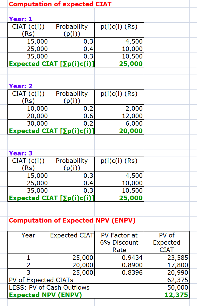
Illustration: 6

A company is considering two mutually exclusive projects X and Y. Project X costs Rs 3, 00,000 and Project Y Rs 3, 60,000. You have been given below the Net Present Value (NPV) probability distribution for each project:

Project X		Project Y
NPV	Probability	NPV	Probability
30,000	0.1	30,000	0.2
60,000	0.4	60,000	0.3
1,20,000	0.4	1,20,000	0.3
1,50,000	0.1	1,50,000	0.2

 

Required:

      1.        Compute the expected net present value of Projects X and Y.

      2.        Compute the risk attached to each project i.e., Standard Deviation of each project.

      3.        Which project do you consider riskier and why?

      4.        Compute the Profitability Index of each project.

 

Solution: 6

Illustration: 7

Skylark Airways is planning to acquire a light commercial aircraft for flying economy class clients at an investment of Rs 50, 00,000. The expected cash flows after tax for the next three years are as follows:

Year: 1		Year: 2		Year: 3
Net cash flows (Rs)	Prob.	Net cash flows (Rs)	Prob.	Net cash flows (Rs)	Prob.
14,00,000	0.1	15,00,000	0.1	18,00,000	0.2
18,00,000	0.2	20,00,000	0.3	25,00,000	0.5
25,00,000	0.4	32,00,000	0.4	35,00,000	0.2
40,00,000	0.3	45,00,000	0.2	48,00,000	0.1

 

The company wishes to take into consideration all possible risk factors relating to an airline operation. The company wants to know:

 

      1.        The Expected NPV of this venture assuming independent probability distribution with 8% risk-free rate of interest, and

      2.        The Standard Deviation of NPV of the venture assuming that the cash flows are uncorrelated.

 

Solution: 7

 

Illustration: 8

A project involves an initial cash outlay of Rs 20,000. The mean or expected value and standard deviation of the cash flows are as follows:

	Year: 1	Year: 2	Year: 3	Year: 4
Expected cash flows (Rs)	10,000	6,000	8,000	6,000
S. D. of cash flows (Rs)	3,000	2,000	4,000	1,200

 

Risk-free rate of interest is 6%. Calculate the expected NPV and S. D. of NPV, if the cash flows of the project are –

     a)        Perfectly correlated, and

     b)        Uncorrelated.

 

Solution: 8

 

Illustration: 9

Cyber Company is considering two mutually exclusive projects. Investment outlay of both the projects is Rs 5, 00,000 and each is expected to have a life of 5 years. Under three possible situations their annual cash flows and probabilities are as follows:

		Cash Flow (Rs)
Situation	Probability	Project: A	Project: B
Good	0.3	6,00,000	5,00,000
Normal	0.4	4,00,000	4,00,000
Worse	0.3	2,00,000	3,00,000

 

If the cost of capital is 9%, which project should be accepted? Explain with workings.

 

Solution: 9

 

Illustration: 10

A project has expected NPV of Rs 800 and S. D. of NPV of Rs 400. The management wants to determine the probability of the NPV in the following ranges:

           (i)        Zero or less.

        (ii)        Greater than zero.

     (iii)        Between the range of Rs 500 and Rs 900.

     (iv)        Between the range of Rs 300 and Rs 600.

 

Solution: 10

 

Illustration: 11

X Ltd. is evaluating an investment proposal which has uncertainty associated with all three major factors: the initial investment or original cost, the useful life and the annual cash flows. The probability distribution of the three variables is as follows:

Original cost		Useful life		Annual CIAT
Rs in lakh	Prob.	Years	Prob.	Rs in lakh	Prob.
9	0.10	7	0.20	2	0.20
7	0.60	6	0.40	2.5	0.40
6	0.30	5	0.40	1.5	0.10
				1	0.30

 

The firm’s risk-free rate of return is 12%. Conduct simulation trials and determine the expected NPV. Also advise on the acceptability of the project.

 

The random numbers are:

Original cost	52	37	82	69	98	96	33	50	88	90
Useful life	6	63	57	2	94	52	69	33	32	30
Annual CIAT	50	28	68	36	90	62	27	50	18	36

 

Solution: 11